The Dilution of Precision – Anchor Geometry
By Lubomir Mraz | June 4th, 2019 | 4 min read
Motivation
When the accuracy of an indoor positioning system comes into play, the anchors’ placement geometry has a key role. It is evaluated via the Dilution of Precision (DOP) mathematical model. It can be applied to all kinds of multilateration systems regardless of the underlying technology or physical phenomena. It does not matter whether the positioning system utilizes radio, ultrasound or light wavelength.
Here, we will be specifically focusing on UWB radio, thanks to its two key features:
- its ability to precisely identify direct signals from reflected ones
- the sub-nano second time-stamping resolution of the incoming signal
On top of this, UWB allows the provision of decimeter-level positioning accuracy immediately at the physical level. This is important because other radio technologies like Wi-Fi and Bluetooth cannot deliver these superior properties. Therefore, they need to be post-processed using additional high-level data wrangling such as incorporating movement-type knowledge, calibration, venue fingerprinting and complicated filtering in order to approach the meter’s level of accuracy. Moreover, all this processing leads to issues with scalability, positioning stability and the limited battery lifetime of tags for such solutions.
We will apply the Time Differential of Arrival (TDoA) positioning technique, which is considered the most scalable approach, allowing the location of thousands of tags in real-time and giving the highest possible battery life.
Let’s take a look at what DOP is. DOP provides a gain factor, which is a dimension-less number – it says how much the position error is amplified at a given point of space by the anchors’ geometry. To make it clear, the distance between anchors does not affect DOP at all. It is just their pure geometry that has an impact.
We will present DOP through examples and it will be calculated within the entire area as a color contour map. The lower the DOP value, the better the accuracy at output.
Practical Deployments
Let’s discuss some deployments of DOP. We will show the most practical, Horizontal DOP (HDOP), since 2D positioning is far more frequent, when compared to 3D positioning, for most applications.
Scenario 1 – Square Anchor Geometry
- Anchors are displaced within a grid of 20 x 20 m at a height of 6 meters – they are indicated with
a red diamond .
. - HDOP is calculated for a tag level of 2 meters.
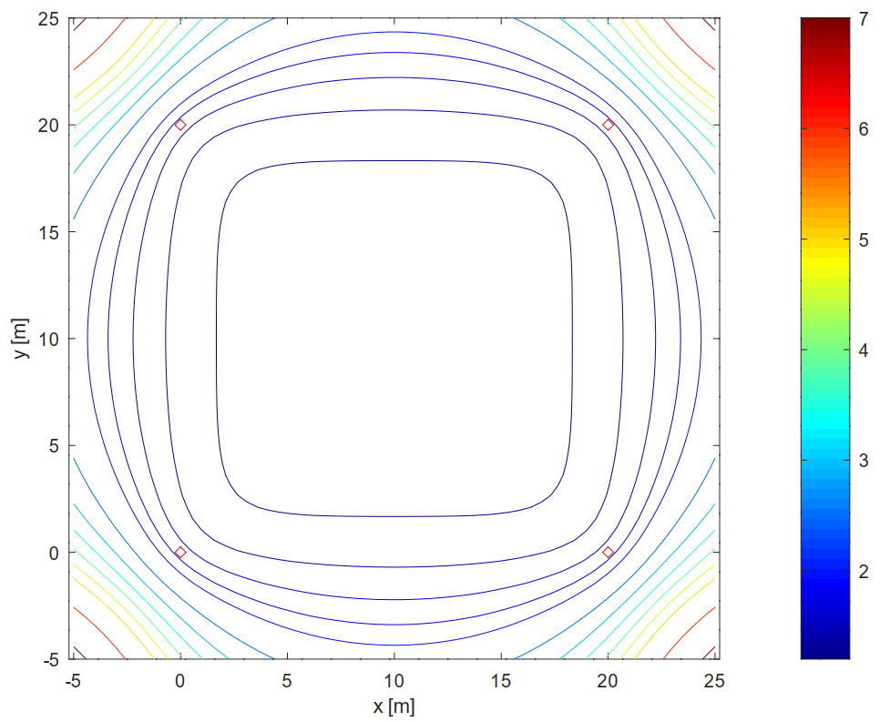
As we can see, the HDOP gain factor values within the inner area are low, which seems to be perfect. Thus, a positioning error should be minimally affected. However, let’s consider the area behind the anchors, the gain values start to become significantly higher.
Let’s compare the inner/outer area in more detail. Here is a simulation for three tags, note the three point clusters in the picture below. Each cluster has a 500 positioning so you can see the corresponding position displacement for each tag. To illustrate it better, the HDOP gain factor is written for each cluster.
Tags are placed at different positions in the inner area of the anchor’s perimeter.

Positions within the inner area are stable, the gain factor is low.
Tags are placed at different positions in the outer area of the anchor’s perimeter.
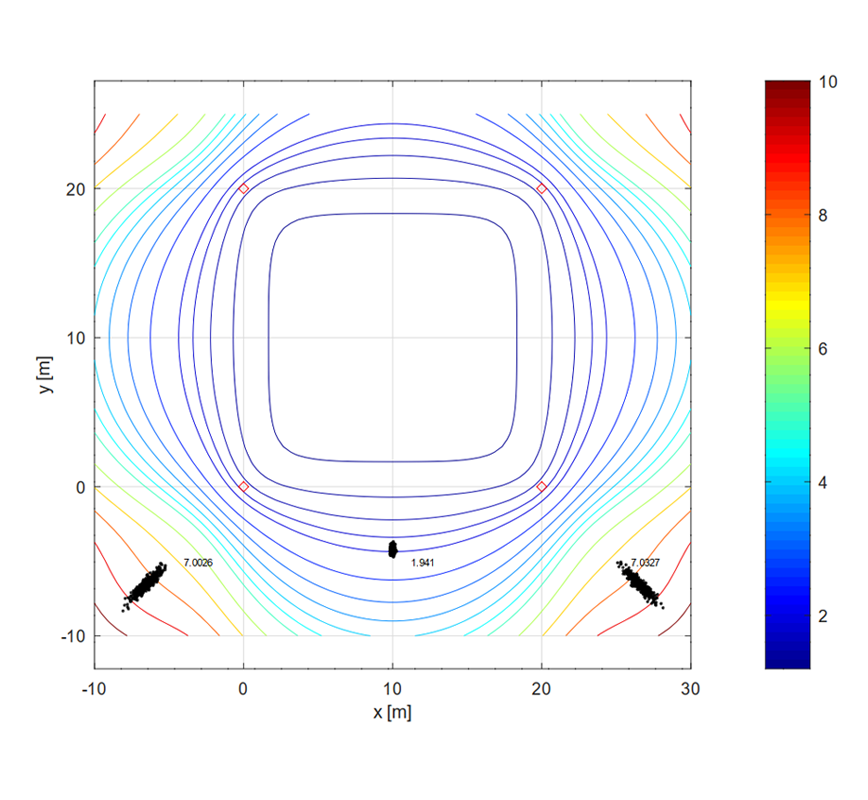
Positions within the outer area report much higher displacement, especially at the corners.
Think about the picking use case. Pallets are placed in the warehouse next to each other with a 0.5 m gap between them.
The goal is to report the correct pallet based on the picking position to WMS. Would you be able to do so if the positions came from the corners beyond the anchor’s perimeter?
One should also consider the virtual zone’s placement with respect to HDOP.
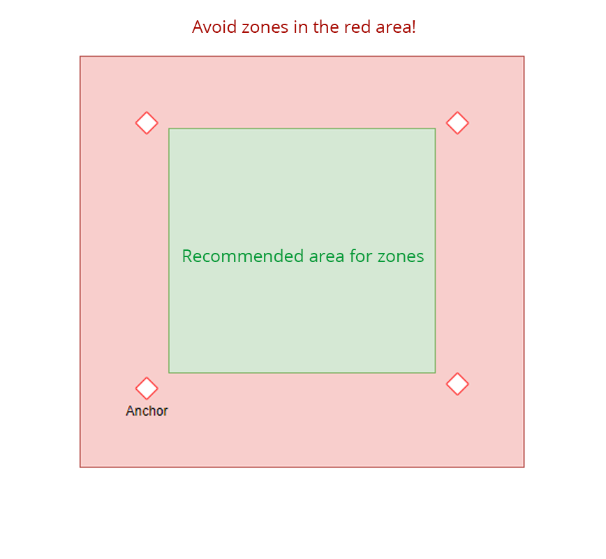
Based on the HDOP displacement from the previous picture, zones should always be created within the inner area, while placing a zone beyond the anchor’s perimeter could cause unwanted zone events as positioning errors increase and confidence levels go down.
Outcome: Anchors should always be placed around the location area. Positions behind anchors should not be used if the given use case cannot tolerate higher positioning displacement.
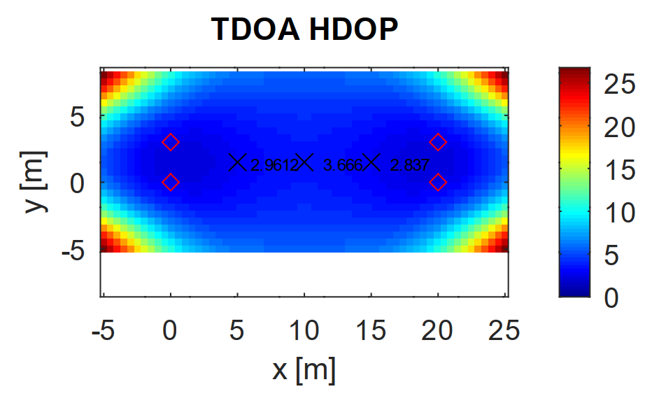
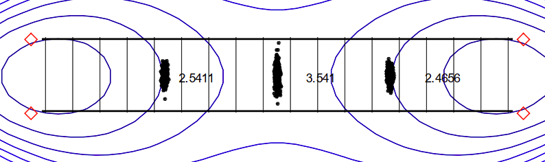
Scenario 2 – Narrow Rectangular Anchor Placement, X:Y Ratio 20:3.
Ok, let’s try to answer another important question, does the x:y ratio between the anchors affect the positioning? Let’s evaluate this on the extreme case of a narrow corridor, for example, in a warehouse.
- Anchors are displaced within a grid of 20 x 3 m at a height of 6 meters, they are indicated with
a red diamond. - HDOP is calculated for a tag level of 2 meters.
- Three tag simulations, each cluster has 500 positions.
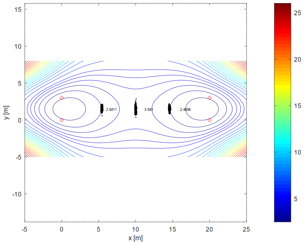
It is obvious that tag positions are more displaced in y-axis than x-axis. HDOP Gain factor values in inner area are between 2 – 4, which is quite high comparing to square deployment above.
Let’s analyze HDOP in more detail – we could divide HDOP into X-axis contribution an Y-axis contribution, see below.
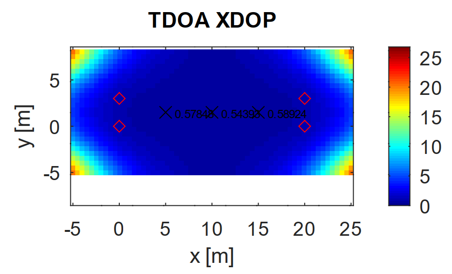
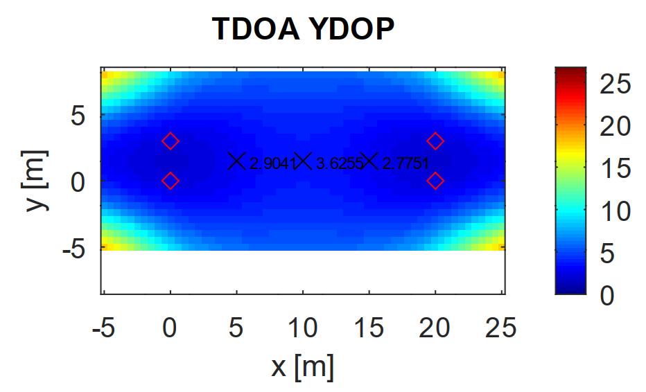
Now, it can be concluded by gain values that position in X-axis (XDOP) is stable, while the most dominant contributor for Tag displacement is in Y-axis (YDOP). Coming back to the use-case with warehouse, positioning system can provide x-axis with high accuracy, but telling whether tag is on top or bottom of the corridor would not be possible.
Outcome
- If X:Y ratio between anchors is too big it amplifies the Tag displacement in given axis.
- Either use-case can tolerate this behavior or more anchors must be placed in order to decrease the X:Y ratio – ideally, we need to squaring the area with anchors to get best DOP.
Grid vs. Keyboard Simplification
Usually, it might be more convenient to simplify the view on HDOP for real use-cases.
One can see the positioning displacement not as a discrete position but as a grid and keyboard:
- grid – for square anchor deployment
- keyboard – for narrow rectangular deployment
Grid Tag Position Displacement
We know that the tag will provide a given accuracy, let’s assume 30 cm, so the location area can be divided by a grid made up of 30 cm squares.
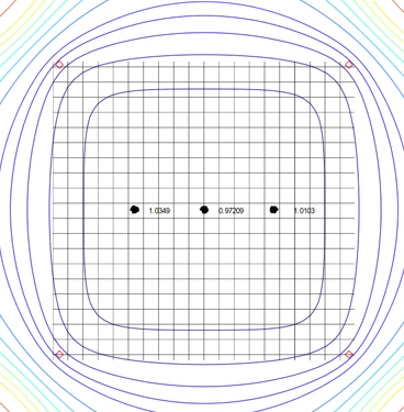
Keyboard Tag Position Displacement
Once the ratio between the anchors becomes highly disproportional, we can see the location area as a keyboard – so we can precisely identify particular keys (x-axis) but we cannot say at which part of the key (y-axis) the tag really is.
Conclusion
It is clear that the correct placement of anchors is crucial to delivering positioning accuracy with a high confidence level. No matter how good the system is on a physical level, its performance can be compromised by incorrect anchor placement!
Therefore:
- If you want to take the guesswork out of designing proper anchor placements before the infrastructure (cabling, holders) is already in place…
- If you are interested in what happens if you add more anchors to different locations…
- If you want to know how much you can decrease the number of anchors by due to the cost restraints…
- If you are curious about how much accuracy is affected by different height levels between tags and anchors…
- If you want to know whether zig-zag anchor deployment can help you and decrease the number of anchors…
Sewio can answer all of these thanks to their advanced training and new RTLS planner tool, where you can DESIGN, SHARE and VALIDATE your deployment. In addition you can OPTIMIZE the system to the lowest possible anchor count necessary!